p5_03 - Train Production Model (deployable)
Step 3 of 3 (final). Load the winning config from
p5_02's YAML artifact. Train the final production model. No HP search, no threshold gymnastics. Fast, deterministic, CI/CD-friendly. This is the deployable artifact - the model you ship to inference services.
1. What we are going to do?
p5_02 discovered the production-ready hyperparameters via GridSearchCV and saved them to artifacts/p5_02_best_config.yaml. This script:
- Reads that YAML config
- Trains the final production model with those exact hyperparameters
- Evaluates on the test set
- Saves the model + metadata to
models/p5_03_production/
That is it. No search. No tuning. No threshold magic. Just train with the known-good config and save.
The production handoff pattern
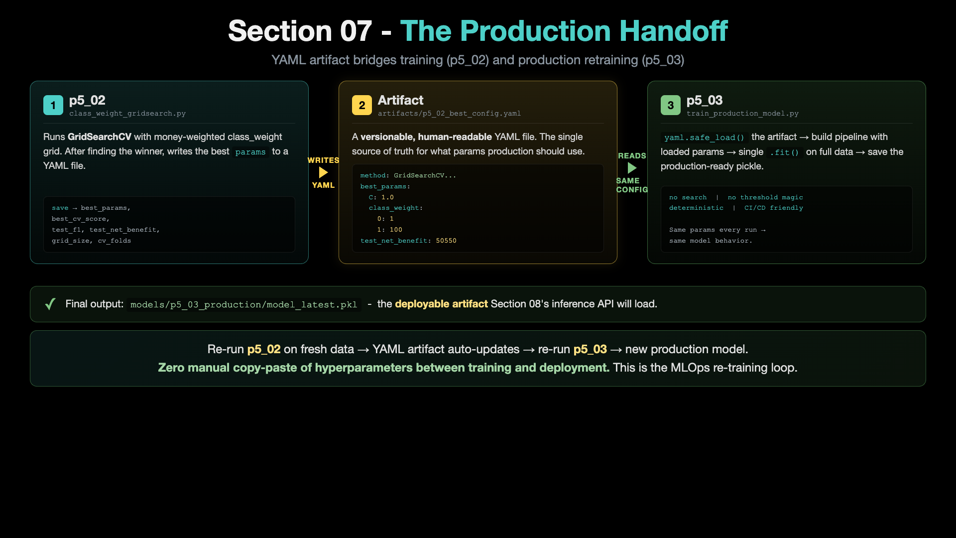
This is the MLOps re-training loop. p5_02 writes artifacts/p5_02_best_config.yaml (left box). p5_03 reads that YAML (right box). The model produced (models/p5_03_production/model_latest.pkl) is what Section 08's inference API loads. Re-run p5_02 on fresh data → YAML auto-updates → re-run p5_03 → new production model. Zero manual copy-paste of hyperparameters between training and deployment.
Why a separate script? In real MLOps you re-train your model regularly (daily / weekly) on fresh data. You do NOT re-run hyperparameter search every time - that is expensive and the result barely changes. Instead, you cache the hyperparameters once (p5_02), and the re-training job (THIS script) just loads them and trains. Re-running p5_02 on fresh data updates the artifact, and the next run of this script automatically picks up the new config.
2. What exactly is it?
The script is purposefully minimal - it does training only. Notable code blocks:
with open(INPUT_ARTIFACT) as f: config = yaml.safe_load(f)- reads the YAML artifactbest_params = config['best_params']- extracts the model params.class_weight={0:1, 1:100}arrives as a dict with int keys, ready to hand to sklearn as-ispipeline = create_pipeline(..., model_params=best_params)- samecreate_pipeline()helper asp3_01/p4_03/p5_01-02pipeline.fit(X_train, y_train)- one train call, no search wrappingpipeline.predict(X_test)- default threshold 0.5 (because the aggressiveness is already baked intoclass_weight)save_pipeline(...)- saves tomodels/p5_03_production/
If p5_02 has not been run, this script errors with a clear message asking you to run it first.
3. How to run it
Step 1 - make sure you are in the mlops-env1 conda environment
Step 2 - go to the project folder
Step 3 - make sure data + FE1 CSV + p5_02 config exist
python p1_01_generate_initial_dataset.py            # only if data does not exist
python p4_01_feature_engineering_fe1.py              # only if FE1 CSV does not exist
python p5_02_class_weight_gridsearch.py              # creates artifacts/p5_02_best_config.yaml
Step 4 - run this script
Runtime: ~2-3 seconds. Just a single model train + test evaluation + save.
4. What is the result output?
The script prints, in order:
- Header banner:
p5_03 - TRAIN PRODUCTION MODEL (uses p5_02 winning config) - STEP 1: loads
artifacts/p5_02_best_config.yamland prints the config
Production config (from p5_02):
  C: 0.1
  l1_ratio: 1.0
  solver: saga
  max_iter: 5000
  class_weight: {0: 1, 1: 100}
(Note: random_state is set internally by create_pipeline() for reproducibility - not part of the search grid, so it does not appear in the loaded config.)
The hyperparameter we inherited from p5_02 - why class_weight={0:1, 1:100} matters
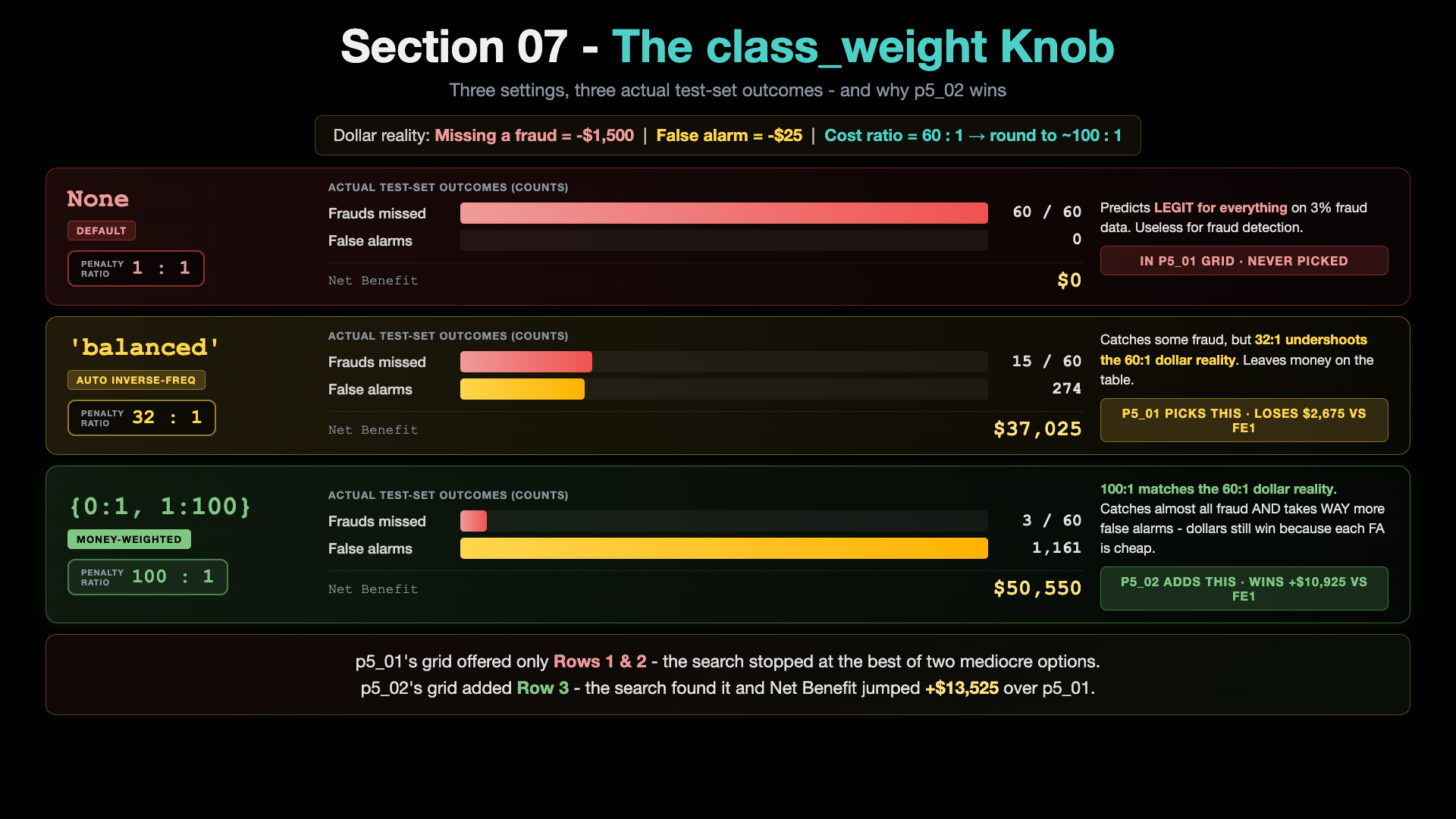
The class_weight={0:1, 1:100} value in the config above is the bottom row of this image (the green one). p5_02 picked it from a 5-value grid because it matches the 60:1 dollar cost ratio of fraud detection. p5_03 just trains with that pre-discovered winner - no search, no second-guessing. This is what "deterministic re-training from a cached config" looks like in practice.
- STEP 2: load FE1 CSV + split
- STEP 3: train production model (no search)
- STEP 4: test-set evaluation block (full
print_metrics()output) - STEP 5: save model + metadata to
models/p5_03_production/ - Closing FULL IMPROVEMENT JOURNEY summary:
FULL IMPROVEMENT JOURNEY (final)
======================================================================

  Stage 1 - Baseline (p3_01, no FE):           $39,625
  Stage 2 - + FE1 (p4_03, amount_ratio):       $39,700   (+$75)
  Stage 3 - + RandomSearch (p5_01):             typically HURT (narrow grid)
  Stage 4 - + GridSearch w/ cw (p5_02):         $50,550   (finds the right params)
  Stage 5 - Production model (p5_03, this):    $50,550

  Total change vs Stage 1 baseline:            +$10,925

  The production model is saved at models/p5_03_production/
  Re-train it any time by re-running p5_02 (updates artifact) then this script.
5. Complete metrics table
For the production model (config inherited from p5_02), evaluated at default threshold 0.5:
| Metric | Value | Note |
|---|---|---|
| F1 Score | 0.0892 | low (same trade-off as p5_02) |
| Precision | 0.0468 | TP / (TP + FP) = 57 / 1,218 |
| Recall | 0.9500 | TP / (TP + FN) = 57 / 60 |
| ROC AUC | 0.8835 | unchanged - threshold-independent |
| Net Benefit | $50,550 | +$10,925 vs baseline ($39,625) |
| Fraud Caught (TP) | 57 / 60 | |
| Fraud Missed (FN) | 3 | only 3 missed out of 60 |
| False Alarms (FP) | 1,161 | high - but $25 each, worth it |
| True Negatives (TN) | 779 |
Metrics match p5_02 exactly because we use the same config on the same train/test split with the same random seed.
Output artifacts: - models/p5_03_production/model_latest.pkl - deployable model - models/p5_03_production/metadata_latest.json - includes best_params, config_source, production_role - results/logistic_regression_p5_03_production_*.json
Where this fits in Section 07
Step 3 of 3. The final deployable. See the section README for the full 3-script arc and the comparison table.
After this section, you have a tuned production model at models/p5_03_production/. Section 08 uses this model to serve predictions via a FastAPI endpoint and compare against the baseline inference API from Section 04.
Prefer to learn by watching?
The video course builds this whole project with you on screen, step by step.