p5_02 - GridSearchCV with money-weighted class_weight
Step 2 of 3.
p5_01's Random search lost money - the search space was too narrow onclass_weight. This script does a properGridSearchCVwith an expanded grid that includes money-weightedclass_weightvalues like{0:1, 1:50}...{0:1, 1:500}. The grid picksclass_weight={0:1, 1:100}and produces Net Benefit $50,550 - +$10,925 over the baseline. Saves the winning config forp5_03(production) to consume.
1. What we are going to do?
p5_01 showed that a generic hyperparameter search can actually HURT - it lost $2,675 versus the FE1 baseline. The miss was the search space itself: it only tried class_weight=['balanced', None], which were not aggressive enough for the cost asymmetry in fraud detection.
This script switches the algorithm from RandomizedSearchCV (what p5_01 used) to GridSearchCV, AND - more importantly - widens the grid to include money-weighted class_weight values. The search:
- Fits the pipeline (preprocessing + LogisticRegression) on
X_train,y_train - Scores each combo by net business value (custom
make_scorer), not by F1 or accuracy - Uses 5-fold cross-validation
- Reports the winning combo
The winning config is saved to artifacts/p5_02_best_config.yaml so p5_03 (production training) can read it without any manual copy-paste between scripts.
Algorithm shift: RandomizedSearchCV → GridSearchCV
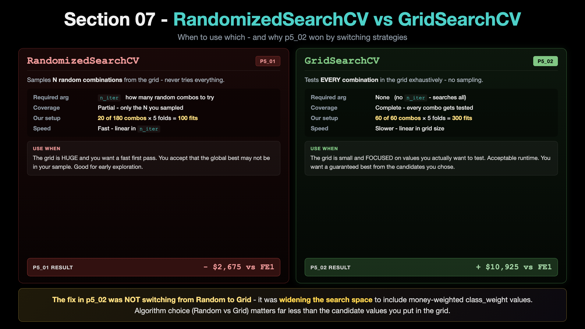
RandomizedSearchCV samples N random combos from a grid (you set n_iter); GridSearchCV tests ALL combos exhaustively. p5_01 used Random because the grid was 180 combos and we did a fast first pass with n_iter=20. p5_02 uses Grid because we've now narrowed the grid down to 60 focused combos - small enough to test exhaustively, and exhaustive testing gives a deterministic winner. But the bigger lesson: algorithm choice (Random vs Grid) is secondary. What unlocked the win was widening the class_weight grid - see the punchline image below.
2. What exactly is it?
A standard GridSearchCV driver. Notable code blocks:
- The search grid expands
p5_01's narrowclass_weightlist to include['balanced', {0:1, 1:30}, {0:1, 1:60}, {0:1, 1:100}, {0:1, 1:200}]. Full grid isC: [0.01, 0.1, 1.0, 10.0],l1_ratio: [0, 0.5, 1.0],solver: ['saga'],max_iter: [5000], plus the 5class_weightvalues business_scorer = make_scorer(business_value_scorer, greater_is_better=True)- business metric in the loop, not F1 (same scorer pattern as p5_01)grid_search = GridSearchCV(pipeline, param_grid, scoring=business_scorer, cv=5, n_jobs=-1, verbose=2)- grid is 4 C x 3 l1_ratio x 5 cw = 60 combos x 5-fold CV = 300 fitsgrid_search.fit(X_train, y_train)- typically runs in ~1-3 minutes- The winning combo is printed and saved as YAML
The grid expansion (what specifically changed vs p5_01)
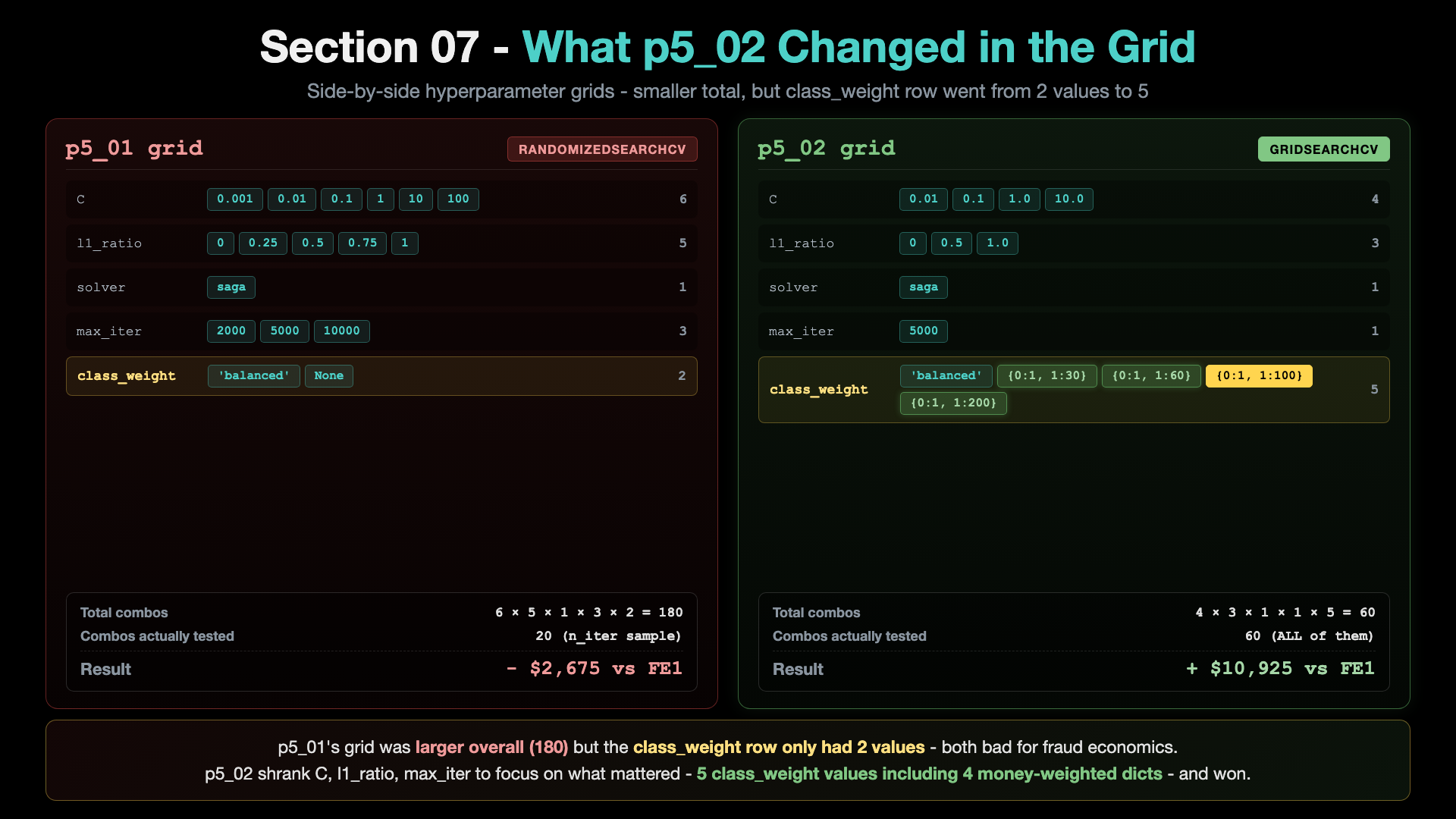
p5_01's grid had class_weight=['balanced', None] (2 values, both bad for the dollar economics). p5_02 keeps 'balanced' but adds 4 money-weighted dicts - including {0:1, 1:100} which matches the 60:1 cost ratio (rounded up). p5_02 also trimmed C, l1_ratio, max_iter ranges to keep the grid focused on what matters. Net effect: smaller TOTAL grid (60 vs 180 in p5_01) but the WINNING value is now IN the grid.
Where class_weight='balanced' actually comes from (the 32:1 derivation)
In Sections 4, 5, and 6 we used class_weight='balanced' in every training script (p3_01, p4_03) and promised to explain WHERE that 32:1 ratio actually comes from when we got to Hyperparameter Tuning. Here is the answer.
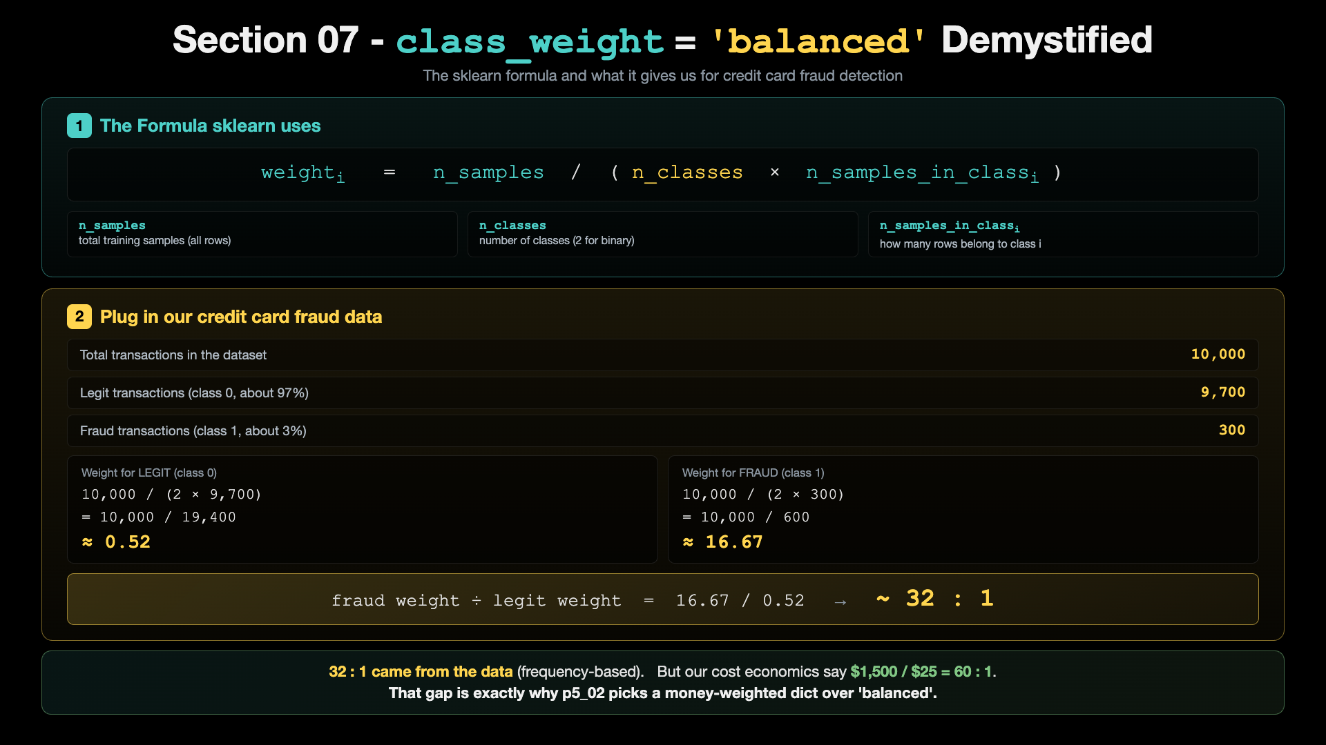
The top half is the sklearn formula: weight_i = n_samples / (n_classes × n_samples_in_class_i). The bottom half plugs in our actual data (10,000 transactions, 9,700 legit, 300 fraud) and computes the two class weights - about 0.52 for legit, about 16.67 for fraud. Divide one by the other and you get the 32:1 ratio.
That 32 is not a choice we made. It comes directly from the class frequencies in the training data. If our fraud rate were 1%, the ratio would jump to about 100. If our fraud rate were 10%, it would drop to about 10. The number is a function of the dataset, not a hyperparameter we tune.
The catch: 32:1 matches the FREQUENCY asymmetry of fraud vs legit. But our cost economics say $1,500 / $25 = 60:1. The two numbers do not agree. That gap is exactly why p5_02 picks a money-weighted dict over 'balanced' - we want to match the COST asymmetry, not the frequency one.
Why money-weighted class_weight wins (THE punchline of Section 07)
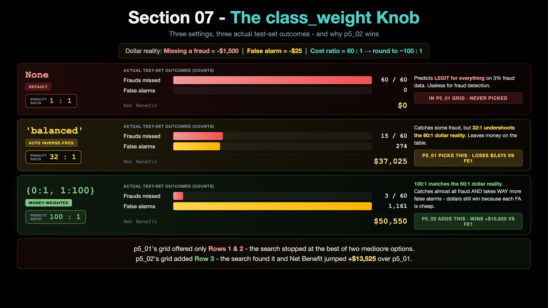
class_weight=None gives a 1:1 penalty ratio (model predicts LEGIT for everything, useless). class_weight='balanced' gives a 32:1 ratio (better but undershoots the dollar reality - see the formula image above). class_weight={0:1, 1:100} gives a 100:1 ratio that MATCHES the actual cost economics (missing fraud $1,500 vs false alarm $25 = 60:1, rounded to 100). p5_01's grid had Rows 1 and 2 only - it lost. p5_02's grid adds Row 3 - it wins.
The 300 fits math
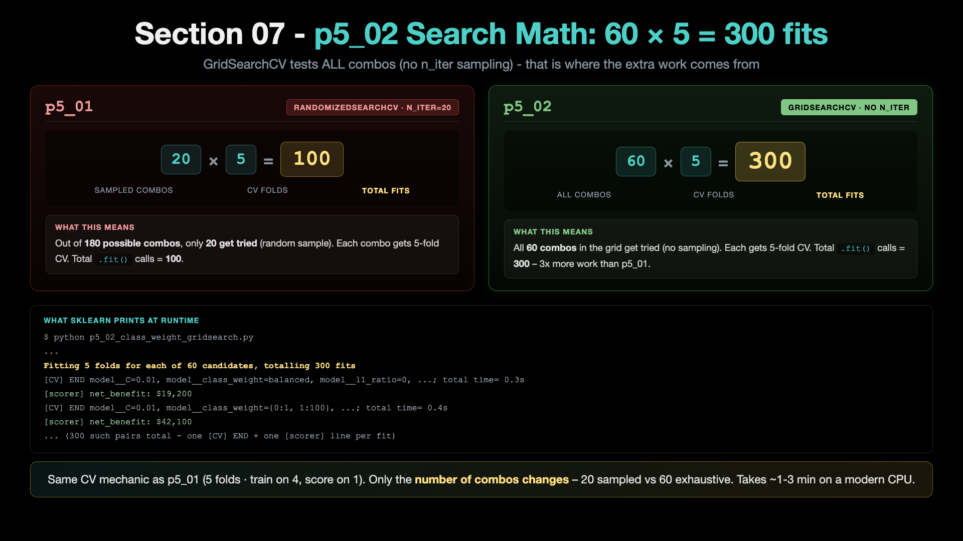
GridSearchCV with our 60-combo grid runs 60 × 5 = 300 model fits (no n_iter to limit it - it tests everything). That is 3x more work than p5_01's 100 fits, but only 60 unique combos (vs p5_01's 180 unique combos with 20 sampled randomly). The takeaway: GridSearch trades MORE work per combo for COMPLETE coverage of a SMALLER focused grid.
Why this matters for the section's narrative
p5_01 showed "generic HP search fails." p5_02 shows "armed with the right search space, the standard search machinery succeeds." This is the actual lesson - search space matters more than search algorithm.
Output artifact for p5_03
The script saves artifacts/p5_02_best_config.yaml with the full best params and the test-set Net Benefit. p5_03 reads this file and trains the production model from it. No manual copy-paste from console output to source code.
YAML is the format for this artifact because class_weight={0:1, 1:100} is a dict with integer keys, and YAML stores int keys natively - the dict round-trips between p5_02 and p5_03 exactly as sklearn expects it.
3. How to run it
Step 1 - make sure you are in the mlops-env1 conda environment
Step 2 - go to the project folder
Step 3 - make sure data + FE1 CSV exist
python p1_01_generate_initial_dataset.py            # only if data does not exist
python p4_01_feature_engineering_fe1.py              # only if FE1 CSV does not exist
Step 4 - run this script
Runtime: ~1-3 minutes depending on machine. n_jobs=-1 uses all cores.
4. What is the result output?
The script prints, in order:
- Header banner:
p5_02 - GridSearchCV with money-weighted class_weight - STEP 1: data load
- STEP 2: build Pipeline (same
create_pipelinehelper as p3_01 / p4_03 / p5_01) - STEP 3: define business-value scorer (dollars, not F1)
- STEP 4: define the search grid (4 C x 3 l1_ratio x 5 cw = 60 combos)
- STEP 5: run GridSearchCV (~1-3 min, prints best params + best CV score)
- STEP 6: test-set evaluation block (full
print_metrics()output) - STEP 7: save model + metadata + save the best config to
artifacts/p5_02_best_config.yaml - Closing IMPROVEMENT JOURNEY SO FAR summary:
IMPROVEMENT JOURNEY SO FAR
======================================================================

 Stage 1 - Baseline (p3_01, no FE):           Net Benefit=$39,625
 Stage 2 - + FE1 (p4_03, + amount_ratio):     Net Benefit=$39,700
 Stage 3 - + RandomSearch (p5_01):            (failed - too narrow grid)
 Stage 4 - + GridSearch w/ cw (p5_02):        Net Benefit=$50,550   (+$10,850 vs FE1)

 Total change vs Stage 1 baseline:            +$10,925

 p5_02's best config is saved to: artifacts/p5_02_best_config.yaml
 This YAML file is what p5_03 will read to train the production model.

 Run next: python p5_03_train_production_model.py (final deployable model)
The winning config looks like:
best_params = {
    'C': 0.1,
    'l1_ratio': 1.0,
    'solver': 'saga',
    'max_iter': 5000,
    'class_weight': {0: 1, 1: 100},
    'random_state': 42,
}
5. Complete metrics table (test set, default threshold 0.5)
| Metric | Value | Note |
|---|---|---|
| F1 Score | 0.0892 | low - precision dropped because we accept many false alarms |
| Precision | 0.0468 | TP / (TP + FP) = 57 / 1,218 |
| Recall | 0.9500 | TP / (TP + FN) = 57 / 60 |
| ROC AUC | 0.8835 | unchanged - threshold-independent |
| Net Benefit | $50,550 | +$10,925 vs baseline ($39,625) |
| Fraud Caught (TP) | 57 / 60 | catches 11 more than baseline |
| Fraud Missed (FN) | 3 | only 3 missed out of 60 |
| False Alarms (FP) | 1,161 | high - but $25 each, worth it |
| True Negatives (TN) | 779 |
Output artifacts: - models/p5_02_class_weight_gridsearch/model_latest.pkl + metadata - results/logistic_regression_p5_02_*.json - artifacts/p5_02_best_config.yaml - consumed by p5_03
Where this fits in Section 07
Step 2 of 3. The HP search done properly. See the section README for the full 3-script arc and the comparison table.
p5_01- Random search with a too-narrow grid. The puzzle (HP tuning HURTS).p5_03- production model trained from THIS script's saved config. The deployable artifact.
After Section 07 you have a tuned production model saved at models/p5_03_production/. Section 08 uses this model to serve predictions via a FastAPI endpoint and compare against the baseline inference API from Section 04.
Prefer to learn by watching?
The video course builds this whole project with you on screen, step by step.